4 Conditional Expectation and The BLP

One of our most fundamental goals as data scientists is to produce predictions that are good. In this week’s async, we make a statement of performance that we can use to evaluate how good a job a predictor is doing, choosing Mean Squared Error.
With the goal of minimizing \(MSE\) we then present, justify, and prove that the conditional expectation function (the CEF) is the globally best possible predictor. This is an incredibly powerful result, and one that serves as the backstop for every other predictor that you will ever fit, whether that predictor is a “simple” regression, or that predictor is a machine learning algorithms (e.g. a random forest) or a deep learning algorithm. Read that again:
Today’s most advanced machine learning algorithms cannot possibly perform better than the conditional expectation function at making a prediction.
📣 At no time ever will a machine learning algorithm perform better than the conditional expectation. 📣
Why does the CEF do so well? Because it can contain a vast amount of complex information and relationships; in fact, the complexity of the CEF is a product of the complexity of the underlying probability space. If that is the case, then why don’t we just use the CEF as our predictor every time?
Well, this is one of the core problems of applied data science work: we are never given the function that describes the behavior of the random variable. And so, we’re left in a world where we are forced to produce predictions from simplifications of the CEF. A very strong simplification, but one that is useful for our puny human brains, is to restrict ourselves to predictors that make predictions from a linear combination of input variables.
Why should we make such a strong restriction? After all, the conditional expectation function might be a fantastically complex combination of input features, why should we entertain functions that are only linear combinations? Essentially, this is because we’re limited in our ability to reason about anything more complex than a linear combination.
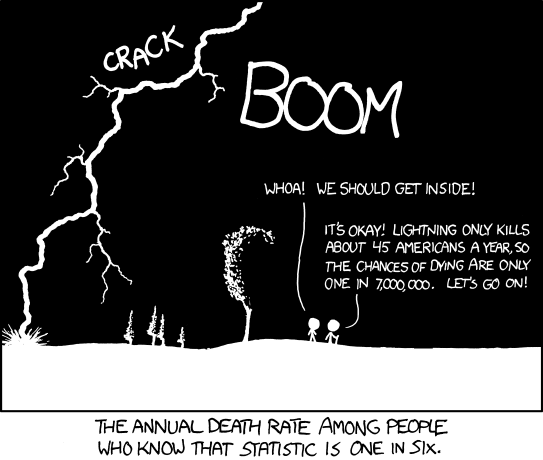
4.1 Thunder Struck
4.2 Learning Objectives
At the end of this weeks learning, which includes the asynchronous lectures, reading the textbook, this live session, and the homework associated with the concepts, student should be able to
- Recognize that the conditional expectation function, the CEF, is a the pure-form, best-possible predictor of a target variable given information about other variables.
- Produce the conditional expectation function as a predictor, given joint densities of random variables.
- Appreciate that the best linear predictor, which is a restriction of predictors to include only those that are linear combinations of variables, can produce reasonable predictions and anticipate that the BLP forms the target of inquiry for regression.
4.3 Class Announcements
4.3.1 Test 1 is releasing to you this week.
The first test is releasing this week. There are review sessions scheduled for this week, practice tests available, and practice problems available. The format for the test is posted in the course discussion channel. In addition to your test, your instructor will describe your responsibilities that are due next week.
4.4 Roadmap
4.4.1 Rearview Mirror
Over the past three weeks, we have talked about how statisticians approach the world, using probability theory to help them make sense of the missing information in the world. This probability theory allows for very general representations of the world; and, if we had the functions that defined the probability distributions, we could do a lot! But, because we don’t live in a simulation (probably…) we don’t have access to the actual functions that describe the probability of events occurring.
We can summarize complex random variables in ways that are useful. We can characterize central tendency using the concept of expected value which is the probability weighted “average” of the outcomes. While there are lots of other ways to characterize central tendency, expectation has some nice properties, namely, that it minimizes mean squared error and also that it is part of the representation of variance. Variance is a measure of dispersion of a random variable, or “how far away from the center” outcomes might occur. It is defined as the probability weighted “average” of the squared deviation. Finally, covariance is a measure of linear dependency between two random variables, and it has a form that is remarkably similar to variance.
4.4.2 This week
- We look at situations with one or more “input” random variables, and one “output.”
- Conditional expectation summarizes the output, given values for the inputs.
- The conditional expectation function (CEF) is a predictor – a function that yields a value for the output, give values for the inputs.
- The best linear predictor (BLP) summarizes a relationship using a line / linear function.
4.4.3 Coming Attractions
- OLS regression is a workhorse of modern statistics, causal analysis, etc
- It is also the basis for many other models in classical stats and machine learning
- The target that OLS estimates is exactly the BLP, which we’re learning about this week.
4.5 Conditional Expectation Function (CEF)
Think back to remember the definition of the expectation of \(Y\):
\[ E[Y] = \int_{-\infty}^\infty y \cdot f_{Y}(y) dy \]
When you read the right hand side of that expectation operator, what are the “ingredients” that are within the integral that produce the expected value? (Hint: there are two.)
This week, the async reading and lectures add a new concept, the conditional expectation of \(Y\) given \(X\):
\[ E[Y|X=x] = \int_{-\infty}^\infty y \cdot f_{Y|X}(y|x) dy \]
When you read the right hand side of that conditional expectation operator, what are the “ingredients” that are within the integral that produce the conditional expected value? (Hint: there are two.)
In what ways are these ingredients similar and in what ways are the different from the expected value above?
4.5.1 Compare Expectation and Conditional Expectation
- Think back by a week: What desirable properties of a predictor does the expectation possess? What makes these properties desirable?
- Think about this week: How, if at all, does the conditional expectation improve on these desirable properties? How does it accomplish this?
4.5.2 Contrast Expectation and Conditional Expectation
Contrast \(E[Y]\) and \(E[Y|X]\). For example, when you look at how these operators are “shaped”, how are their components similar or different?1
What is \(E[Y|X]\) a function of? What are “input” variables to this function?
What, if anything, is \(E[E[Y|X]]\) a function of?
4.6 Computing the CEF
- Suppose that random variables \(X\) and \(Y\) are jointly continuous, with joint density function given by,
\[ f(x,y) = \begin{cases} 2, & 0 \leq x \leq 1, 0 \leq y \leq x \\ 0, & otherwise \end{cases} \]
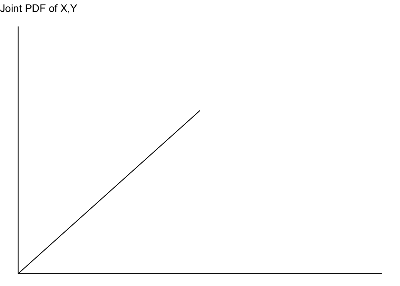
What does the joint PDF of this function look like?
4.6.1 Simple Quantities
To begin with, let’s compute the simplest quantities:
- What is the expectation of \(X\)?
- What is the expectation of \(Y\)?
- How would you compute the variance of \(X\)? (We’re not going to do it live).
4.6.2 Conditional Quantities
4.6.2.1 Conditional Expectation
And then, let’s think about how to compute the conditional quantities.
Compute the \(CEF[Y|X]\). Start by writing down the statement of the conditional expectation function, and then, compute the value.
Once you have computed the \(CEF[Y|X]\), use this function to answer the following questions:
- What is the conditional expectation of \(Y\), given that \(X=x=0\)?
- What is the conditional expectation of \(Y\), given that \(X=x=0.5\)?
- What is the conditional expectation of \(X\), given that \(Y=y=0.5\)?
4.6.2.2 Conditional Variance
- What is the conditional variance function?2
- Which of the two of these has a lower conditional variances?
- \(V[Y|X=0.25]\); or,
- \(V[Y|X=0.75]\).
- How does \(V[Y]\) compare to \(V[Y|X=1]\)? Which is larger?
4.6.3 Conditional Expectation
4.7 Minimizing the MSE
4.7.1 Minimizing MSE
Theorem 2.2.20 states,
The CEF \(E[Y|X]\) is the “best” predictor of \(Y\) given \(X\), where “best” means it has the smallest mean squared error (MSE).
Oh yeah? As a breakout group, ride shotgun with us as we prove that the conditional expectation is the function that produces the smallest possible Mean Squared Error.
Specifically, you group’s task is to justify every transition from one line to the next using concepts that we have learned in the course: definitions, theorems, calculus, and algebraic operations.
4.7.2 The pudding (aka: “Where the proof is”)
We need to find such function \(g(X): \mathbb{R} \to \mathbb{R}\) that gives the smallest mean squared error.
First, let MSE be defined as it is in Definition 2.1.22.
For a random variable \(X\) and constant \(c \in \mathbb{R}\), the mean squared error of \(X\) about \(c\) is \(E[(x-c)^2]\).
Second, let us note that since \(g(X)\) is just a function that maps onto \(\mathbb{R}\), that for some particular value of \(X=x\), \(g(X)\) maps onto a constant value.
- Deriving a Function to Minimize MSE
\[ \begin{aligned} E[(Y - g(X))^2|X] &= E[Y^2 - 2Yg(X) + g^2(X)|X] \\ &= E[Y^2|X] + E[-2Yg(X)|X] + E[g^2(X)|X] \\ &= E[Y^2|X] - 2g(X)E[Y|X] + g^2(X)E[1|X] \\ &= (E[Y^2|X] - E^2[Y|X]) + (E^2[Y|X] - 2g(X)E[Y|X] + g^2(X)) \\ &= V[Y|X] + (E^2[Y|X] - 2g(X)E[Y|X] + g^2(X)) \\ &= V[Y|X] + (E[Y|X] - g(X))^2 \\ \end{aligned} \]
Notice too that we can use the Law of Iterated Expectations to do something useful. (This is a good point to talk about how this theorem works in your breakout groups.)
\[ \begin{aligned} E[(Y-g(X))^2] &= E\big[E[(Y-g(X))^2|X]\big] \\ &=E\big[V[Y|X]+(E[Y|X]-g(X))^2\big] \\ &=E\big[V[Y|X]\big]+E\big[(E[Y|X]-g(X))^2\big]\\ \end{aligned} \]
- \(E[V[Y|X]]\) doesn’t depend on \(g\); and,
- \(E[(E[Y|X]-g(X))^2] \geq 0\).
\(\therefore g(X) = E[Y|X]\) gives the smallest \(E[(Y-g(X))^2]\)
4.7.3 The Implication
If you are choosing some \(g\), you can’t do better than \(g(x) = E[Y|X=x]\).
4.7.4 Working with a gnarly function and a lot of data.
This is risky, because it makes you want data, and we don’t get it yet. We haven’t earned our stripes and we’re still figuring out what works in the perfect world of the population rather than the grimy world of data. 🤫
dat |>
  ggplot() +
  aes(x = x, y = y) +
  geom_point(alpha=0.25, size=.1)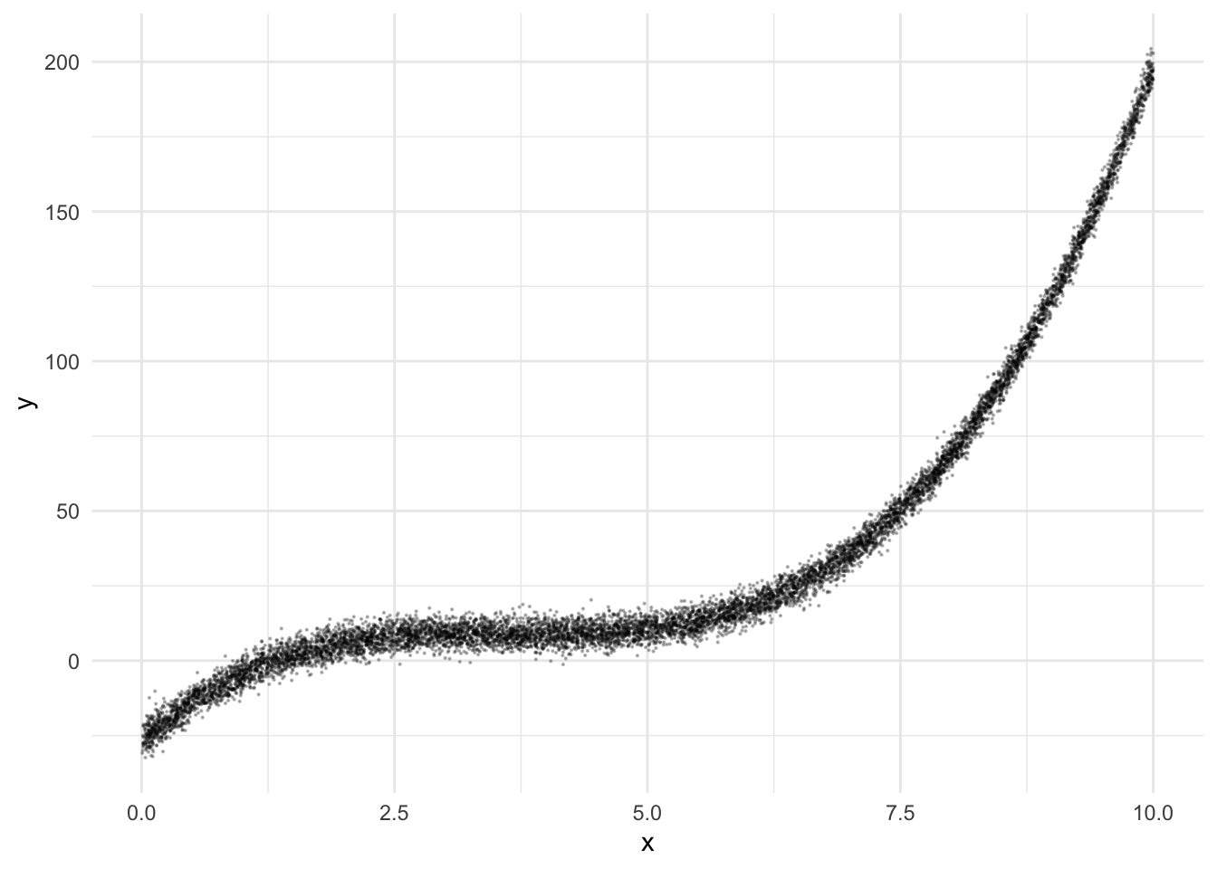
l <- loess(y ~ x, data = dat, span = .1)
# ask for student prediction functions
mod_lm   <- lm(y ~ x, data = dat)
mod_lm_2 <- lm(y ~ poly(x, 2), data = dat)
mod_lm_3 <- lm(y ~ poly(x, 3), data = dat)

predict.lm(mod_lm, newdata = data.frame(x))[1:10]
1 2 3 4 5 6 7
48.324031 51.067296 -23.603841 49.905316 15.836212 18.641871 24.513068
8 9 10
46.456447 5.331306 -5.891294 dat <- dat |>
mutate(
pred_loess = predict(l, x),
pred_lm = as.numeric(predict(mod_lm)),
pred_lm_2 = as.numeric(predict(mod_lm_2)),
pred_lm_3 = as.numeric(predict(mod_lm_3))
## fill student prdictions here
)
dat |> head() x y pred_loess pred_lm pred_lm_2 pred_lm_3
1 7.092161 34.81333880 36.2546940 48.32403 49.864735 38.2119682
2 7.312937 38.34412765 43.2961525 51.06730 55.423279 44.3393578
3 1.303471 -25.62406387 0.2663361 -23.60384 2.792496 -0.1589276
4 7.219422 24.81035757 39.6432863 49.90532 53.035060 41.6497067
5 4.477571 -1.74494571 8.4743358 15.83621 5.063831 9.2218484
6 4.703368 0.06490843 7.9944393 18.64187 7.402918 9.6026823Let’s pull in a mean squared error function:
mse <- function(truth, prediction) {
  mse_ <- mean((truth - prediction)^2)
  return(mse_)
}mse(truth = dat$y, prediction = dat$pred_loess)[1] 884.9086mse(truth = dat$y, prediction = dat$pred_lm)[1] 1351.689mse(truth = dat$y, prediction = dat$pred_lm_2)[1] 1093.046mse(truth = dat$y, prediction = dat$pred_lm_3)[1] 886.9722dat |>
ggplot() +
aes(x = x, y = y) +
geom_point(alpha=0.25, size=.1) +
geom_line(aes(x = x, y = pred_loess), color = "darkred") +
geom_line(aes(x = x, y = pred_lm), color = "darkblue") +
geom_line(aes(x = x, y = pred_lm_2), color = "darkorange") +
geom_line(aes(x = x, y = pred_lm_3), color = "darkgreen")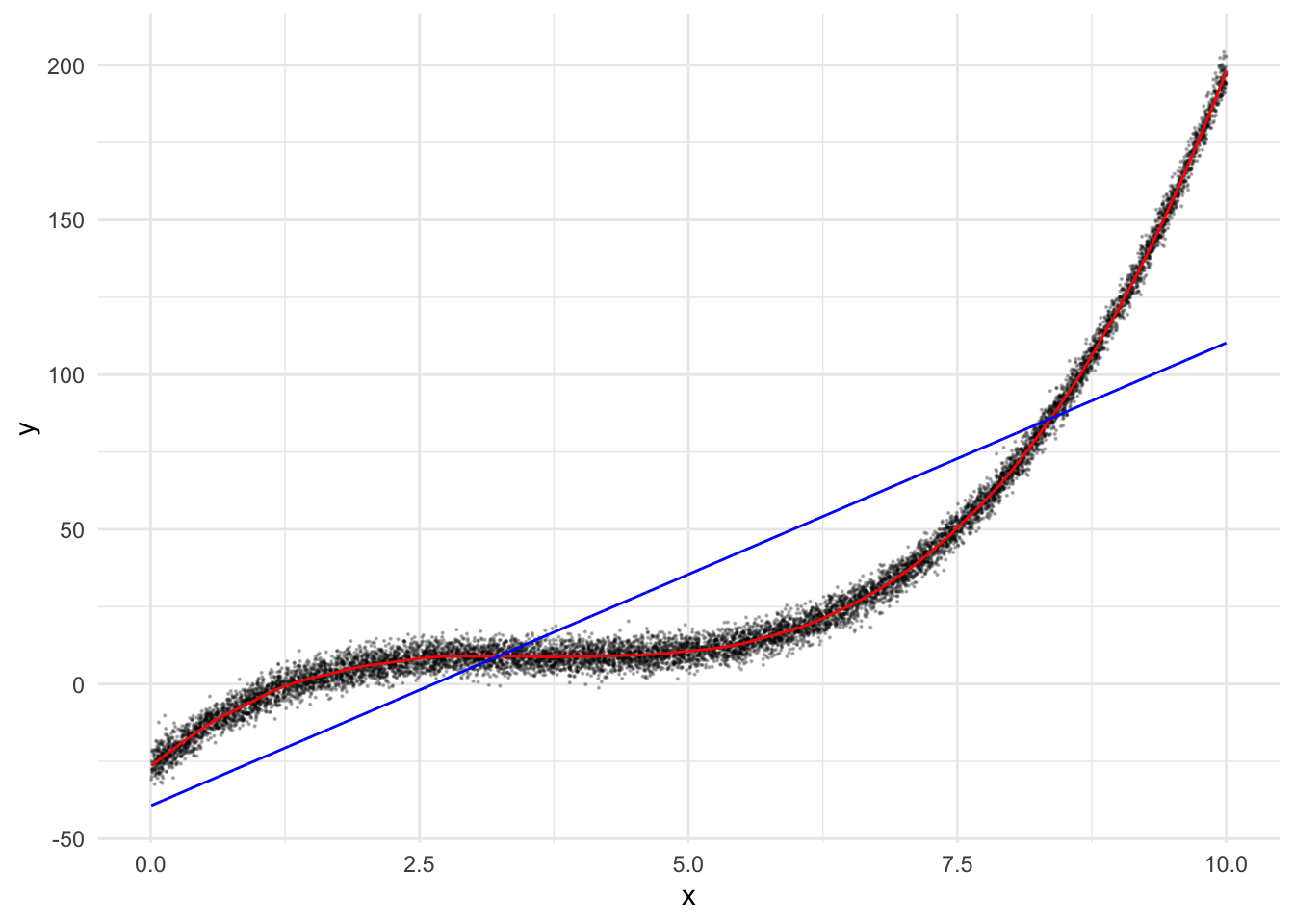
What would happen if, rather than having this much data, you had much much less?
dat_small <- dat |>
  slice_sample(n = 20) |>
  add_row(x=5, y=50) |>
  arrange(x)

mod_l_small    <- loess(formula = y ~ x, span = .1, data = dat_small)
mod_lm_small   <- lm(formula = y ~ x, data = dat_small)
mod_lm_2_small <- lm(y ~ poly(x, 2), data = dat_small)
mod_lm_3_small <- lm(y ~ poly(x, 3), data = dat_small)

dat_small <- dat_small |>
  mutate(
    pred_loess_small = predict(mod_l_small),
    pred_lm_small    = predict(mod_lm_small),
    pred_lm_2_small  = predict(mod_lm_2_small),
    pred_lm_3_small  = predict(mod_lm_3_small)
  )

dat <- dat |>
  mutate(
    pred_loess_small = predict(mod_l_small, newdata = dat$x),
    pred_lm_small    = predict(mod_lm_small, newdata = dat),
    pred_lm_2_small  = predict(mod_lm_2_small, newdata = dat),
    pred_lm_3_small  = predict(mod_lm_3_small, newdata = dat)
  )

dat |>
  ggplot() +
  geom_line(aes(x = x, y = pred_loess_small), color = "darkred") +
  geom_line(aes(x = x, y = pred_lm_small),    color = "darkblue") +
  geom_line(aes(x = x, y = pred_lm_2_small),  color = "darkorange") +
  geom_line(aes(x = x, y = pred_lm_3_small),  color = "darkgreen") +
  geom_point(aes(x = dat$x, y = dat$y), size=.1, alpha=.1)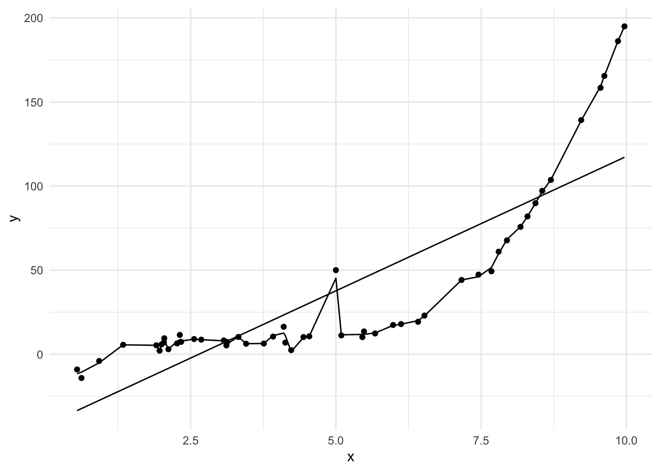
4.8 Working with the BLP
Why Linear?
- In some cases, we might try to estimate the CEF. More commonly, however, we work with linear predictors. Why?
- We don’t know joint density function of \(Y\). So, it is “difficult” to derive a suitable CEF.
- To estimate flexible functions requires considerably more data. Assumptions about distribution (e.g. a linear form) allow you to leverage those assumptions to learn ‘more’ from the same amount of data.
- Other times, the CEF, even if we could produce an estimate, might be so complex that it isn’t useful or would be difficult to work with.
- And, many times, linear predictors (which might seem trivially simple) actually do a very good job of producing predictions that are ‘close’ or useful.
4.8.1 Continuous BLP
- Recall the PDF that we worked with earlier to produce the \(CEF[Y|X]\).
\[ f(x,y) = \begin{cases} 2, & 0 \leq x \leq 1, 0 \leq y \leq x \\ 0, & otherwise \end{cases} \]
Find the \(BLP\) for \(Y\) as a function of \(X\). What, if anything, do you notice about this \(BLP\) and the \(CEF\)?
Note, when we say “shaped” here, we’re referring to the deeper concept of a statistical functional. A statistical functional is a function of a function that maps to a real number. So, if \(T\) is the functional that we’re thinking of, \(\mathcal{F}\) is a family of functions that it might operate on, and \(\mathbb{R}\) is the set of real numbers, a statistical functional is just \(T: \mathcal{F} \rightarrow \mathbb{R}\). The Expectation statistical functional, \(E[X]\) always has the form \(\int x f_{X}(x)dx\).)↩︎
Take a moment to strategize just a little bit before you get going on this one. There is a way to compute this value that is easier than another way to compute this value.↩︎