10.5 R Activity: Measuring the return to education

In labor economics, a key concept is returns to education.
Our goal is description: what is the relationship between education and wages? We will proceed in two steps:
- First, we will discuss what the appropriate specifications are.
- Then we will estimate the different models to answer this question.
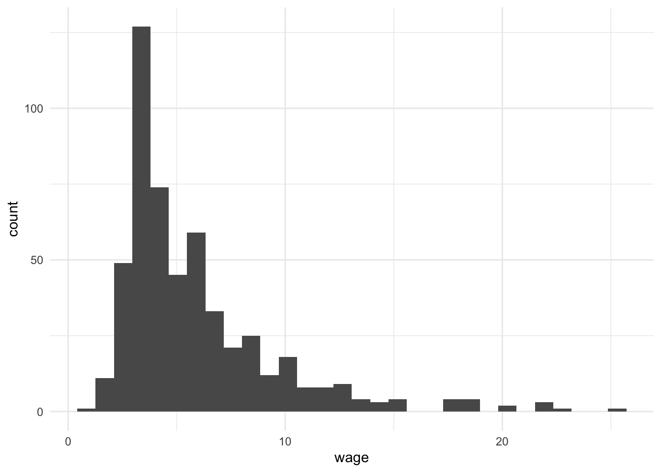
We will use wage1 dataset in the wooldridge package in the following sections.

Code

wage1 <- wooldridge::wage1
#names(wage1)

wage1 %>% 
  ggplot() + 
  aes(x=wage) + 
  geom_histogram()

## `stat_bin()` using `bins = 30`. Pick better value with `binwidth`.

Which of the following specifications best capture the relationship between education and hourly wage? (Hint: Do a quick a EDA)
- level-level: \(wage = \beta_0 + \beta_1 educ + u\)
- Level-log: \(wage = \beta_0 + \beta_1 \ln(educ) + u\)
- log-level: \(\ln(wage) = \beta_0 + \beta_1 educ + u\)
- log-log: \(\ln(wage) = \beta_0 + \beta_1 \ln(educ) + u\)
What is the interpretation of \(\beta_0\) and \(\beta_1\) in your selected specification?
Can we use \(R^2\) or Adjusted \(R^2\) to choose between level-level or log-level specifications?

Remember

Doing a log transformation for any reason essentially implies a fundamentally different relationship between outcome (Y) and predictor (X) that we need to capture

The following specifications include two control variables: years of experience (exper) and years at current company (tenure).
Do a quick EDA and select the specification that better suits our description goal.
- \(wage = \beta_0 + \beta_1 educ + \beta_2 exper + \beta_3 tenure + u\)
- \(\begin{aligned} wage &= \beta_0 + \beta_1 educ + \beta_2 exper + \beta_3 exper^2 + \\ & \beta_4 tenure + \beta_5 tenure^2 + u \end{aligned}\)
How do you interpret the \(\beta\) coefficients?

In the following models, first, explain why the indicator variables or interaction terms have been included. Then identify the reference group (if any) and interpret all coefficients.
- \(wage = \beta_0 + \beta_1 educ + \beta_2 I(educ \geq 12) + u\)
- \(wage = \beta_0 + \beta_1 educ + \beta_2 female + u\)
- \(wage = \beta_0 + \beta_1 educ + \beta_2 female + \beta_3 educ*female + u\)
- \(\begin{aligned} wage &= \beta_0 + \beta_1 female + \beta_2 I(educ = 2) + \beta_3 I(educ = 3)\\ &...+ \beta_{20} I(educ = 20) + u\\ \end{aligned}\)

Estimating Returns to Education

Answer the following questions using an appropriate hypothesis test.
1. Is a year of education associated with changes to hourly wage? (Include experience and tenure without polynomial terms).
2. Is the association between wage and experience / wage and tenure non-linear?
3. Is there evidence for gender wage discrimination in the U.S.?
4. Is there any evidence for a graduation effect on wage?
Display all estimated models in a regression table, and discuss the robustness of your results.