9.5 Understanding Uncertainty

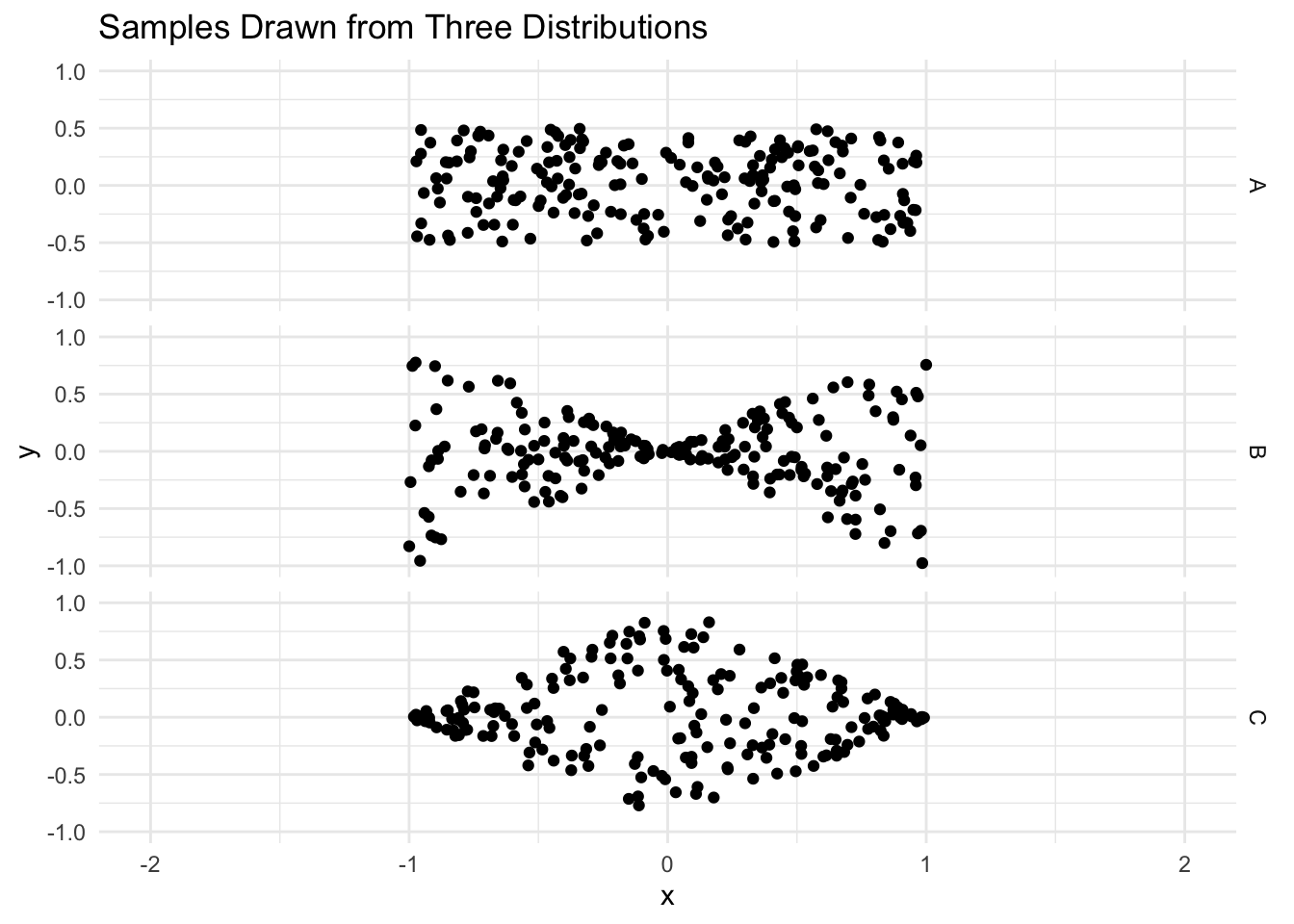
Imagine three different regression models, each of the following form:

\[ Y = 0 + \beta X + \epsilon \]

The only difference is in the error term. The conditional distribution is given by:

Model	Distribution of \(\epsilon\) cond. on \(X\)
A	Uniform on \([-.5, +.5]\)
B	Uniform on \([ - |X|, |X| ]\)
C	Uniform on \([ -1 + |X|, 1- |X| ]\)

A is what we call a homoskedastic distribution. B and C are what we call heteroskedastic. Below, we define R functions that simulate draws from these three distributions.

Code

rA <- function(n, slope=0){
  x       = runif(n, min=-1, max = 1)
  epsilon = runif(n, min=-.5, max=.5)
  y       = 0 + slope*x + epsilon
  return( data.frame(x=x,y=y) )
}

rB <- function(n, slope=0){
  x       = runif(n, min=-1, max = 1)
  epsilon = runif(n, min=- abs(x), max=abs(x))
  y       = 0 + slope*x + epsilon
  return( data.frame(x=x,y=y) )
}

rC <- function(n, slope=0){
  x       = runif(n, min=-1, max = 1)
  epsilon = runif(n, min= -1 + abs(x), max=1 - abs(x))
  y       = 0 + slope*x + epsilon
  return( data.frame(x=x,y=y) )
}

Code

data <- rbind( 
  data.frame( rA(200), label = 'A'),
  data.frame( rB(200), label = 'B'),
  data.frame( rC(200), label = 'C'))

Code

data %>% 
  ggplot(aes(x=x, y=y)) + 
  geom_point() + 
  lims(
    x = c(-2,2), 
    y = c(-1,1)) + 
  labs(title = 'Samples Drawn from Three Distributions') + 
  facet_grid(rows=vars(label))

9.5.1 Question 1

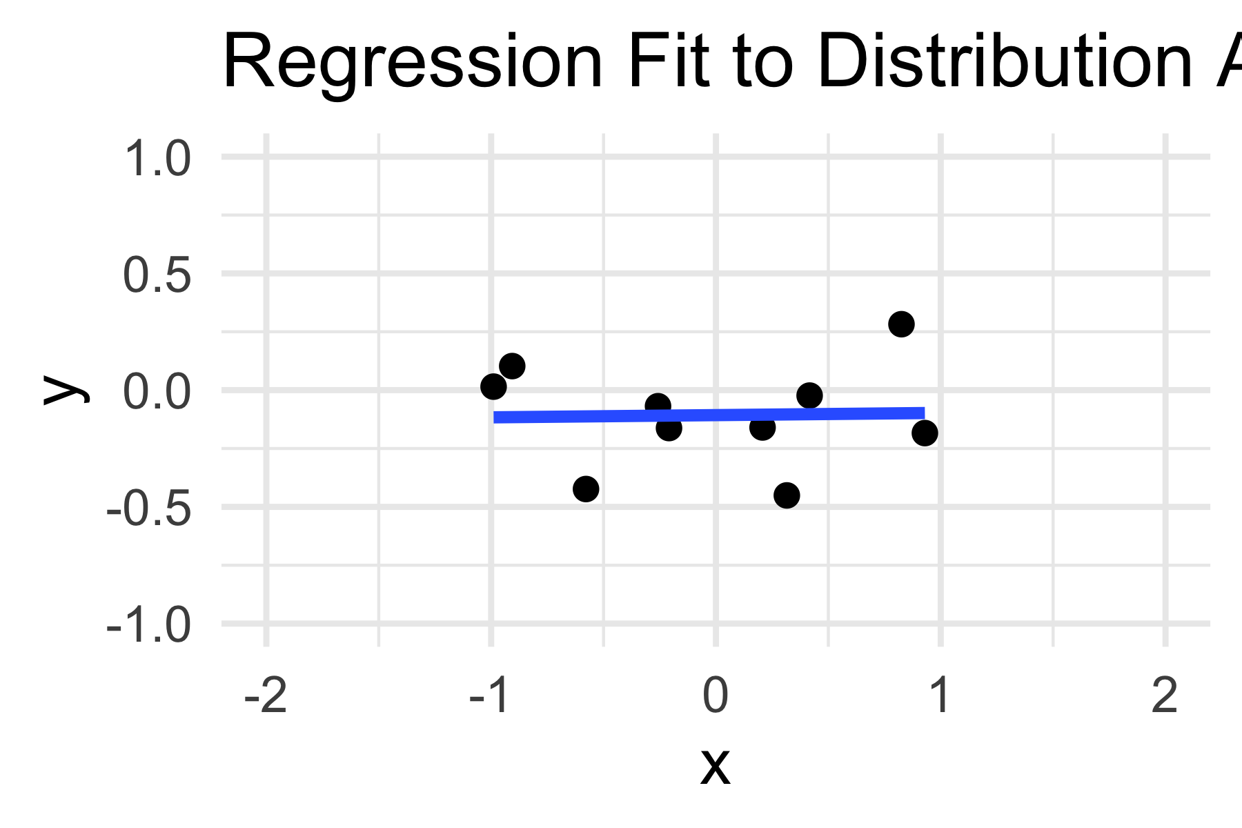
The following code draws a sample from distribution A, fits a regression line, and plots it. Run it a few times to see what happens. Now explain how you would visually estimate the standard error of the slope coefficient. Why is this standard error important?

Code

data <-  rA(10, slope=0)

data %>% 
  ggplot() + 
  aes(x=x, y=y) + 
  geom_point() + 
  geom_smooth(method='lm', formula = 'y ~ x', se=FALSE) + 
  lims(
    x = c(-2,2), 
    y = c(-1,1)) + 
  labs(title = 'Regression Fit to Distribution A')

Code

data_points <- 200

base_plot_a <- rA(10) %>%  
  ggplot() + 
  aes(x=x, y=y) + 
  geom_point() + 
  scale_x_continuous(limits = c(-3, 3))

for(i in 1:100) { 
    base_plot_a <- base_plot_a + rA(data_points) %>% 
      stat_smooth(
        mapping = aes(x=x, y=y), 
        method  = 'lm',         se = FALSE, 
        formula = 'y~x', fullrange = TRUE,
        color   = 'grey',    alpha = 0.5,
        size    = 0.5
      )
}

## Warning: Using `size` aesthetic for lines was deprecated in ggplot2 3.4.0.
## ℹ Please use `linewidth` instead.
## This warning is displayed once every 8 hours.
## Call `lifecycle::last_lifecycle_warnings()` to see where this warning was generated.

Code

base_plot_b <- rB(10) %>%  
  ggplot() + 
  aes(x=x, y=y) + 
  geom_point() + 
  scale_x_continuous(limits = c(-3, 3))

for(i in 1:100) { 
    base_plot_b <- base_plot_b + rB(data_points) %>% 
      stat_smooth(
        mapping = aes(x=x, y=y), 
        method  = 'lm',         se = FALSE, 
        formula = 'y~x', fullrange = TRUE,
        color   = 'grey',    alpha = 0.5,
        size    = 0.5
      )
  }

base_plot_c <- rC(10) %>%  
  ggplot() + 
  aes(x=x, y=y) + 
  geom_point() + 
  scale_x_continuous(limits = c(-3, 3))

for(i in 1:100) { 
    base_plot_c <- base_plot_c + rC(data_points) %>% 
      stat_smooth(
        mapping = aes(x=x, y=y), 
        method  = 'lm',         se = FALSE, 
        formula = 'y~x', fullrange = TRUE,
        color   = 'grey',    alpha = 0.5,
        size    = 0.5
      )
}

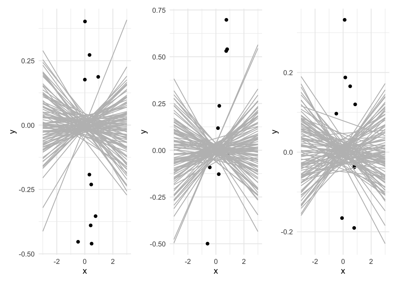
base_plot_a | base_plot_b  | base_plot_c

9.5.2 Question 2

You have a sample from each distribution, A, B, and C and you fit a regression of Y on X. Which will have the highest standard error for the slope coefficient? Which will have the lowest standard error? Why? (You may want to try experimenting with the function defined above)

9.5.3 Question 3

For distribution A, perform a simulated experiment. Draw a large number of samples, and for each sample fit a linear regression. Store the slope coefficient from each regression in a vector. Finally, compute the standard deviation for the slope coefficients.

Repeat this process for distributions B and C. Do the results match your intuition?