12.5 R Exercise

Code

library(tidyverse)
library(wooldridge)
library(car)
library(lmtest)
library(sandwich)
library(stargazer)

If you haven’t used the mtcars dataset, you haven’t been through an intro applied stats class!

In this analysis, we will use the mtcars dataset which is a dataset that was extracted from the 1974 Motor Trend US magazine, and comprises fuel consumption and 10 aspects of automobile design and performance for 32 automobiles (1973-74 models). The dataset is automatically available when you start R.

For more information about the dataset, use the R command: help(mtcars)

Code

data(mtcars)
glimpse(mtcars)

## Rows: 32
## Columns: 11
## $ mpg  <dbl> 21.0, 21.0, 22.8, 21.4, 18.7, 18.1, 14.3, 24.4, 22.8, 19.2, 17.8,…
## $ cyl  <dbl> 6, 6, 4, 6, 8, 6, 8, 4, 4, 6, 6, 8, 8, 8, 8, 8, 8, 4, 4, 4, 4, 8,…
## $ disp <dbl> 160.0, 160.0, 108.0, 258.0, 360.0, 225.0, 360.0, 146.7, 140.8, 16…
## $ hp   <dbl> 110, 110, 93, 110, 175, 105, 245, 62, 95, 123, 123, 180, 180, 180…
## $ drat <dbl> 3.90, 3.90, 3.85, 3.08, 3.15, 2.76, 3.21, 3.69, 3.92, 3.92, 3.92,…
## $ wt   <dbl> 2.620, 2.875, 2.320, 3.215, 3.440, 3.460, 3.570, 3.190, 3.150, 3.…
## $ qsec <dbl> 16.46, 17.02, 18.61, 19.44, 17.02, 20.22, 15.84, 20.00, 22.90, 18…
## $ vs   <dbl> 0, 0, 1, 1, 0, 1, 0, 1, 1, 1, 1, 0, 0, 0, 0, 0, 0, 1, 1, 1, 1, 0,…
## $ am   <dbl> 1, 1, 1, 0, 0, 0, 0, 0, 0, 0, 0, 0, 0, 0, 0, 0, 0, 1, 1, 1, 0, 0,…
## $ gear <dbl> 4, 4, 4, 3, 3, 3, 3, 4, 4, 4, 4, 3, 3, 3, 3, 3, 3, 4, 4, 4, 3, 3,…
## $ carb <dbl> 4, 4, 1, 1, 2, 1, 4, 2, 2, 4, 4, 3, 3, 3, 4, 4, 4, 1, 2, 1, 1, 2,…

12.5.1 Questions:

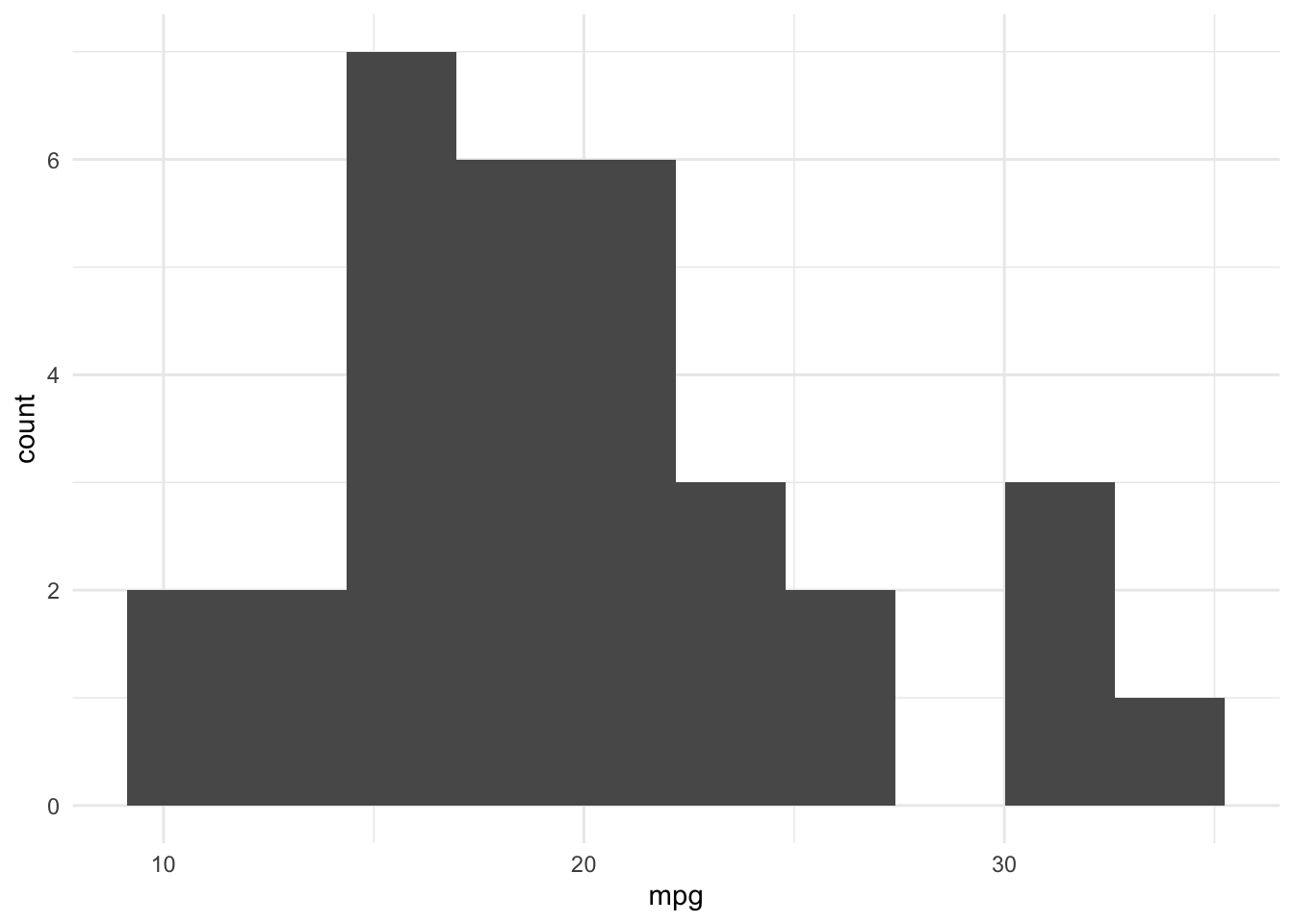
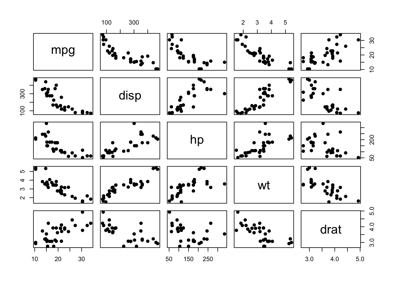
0. Using the mtcars data, quickly reason about the variables that we’re interested in studying:

Code

mtcars %>% 
  ggplot() + 
  aes(x=mpg) +
  geom_histogram(bins=10)

Code

mtcars %>% 
  select(mpg, disp, hp, wt, drat) %>% 
  pairs(pch=19)

1. Using the mtcars data, run a linear regression to find the relationship between miles per gallon (mpg) on the left-hand-side as a function of displacement (disp), gross horsepower (hp), weight (wt), and rear axle ratio (drat) on the right-hand-side. That is, fit a regression of the following form:

\[ \widehat{mpg} = \hat{\beta_{0}} + \hat{\beta}_{1} disp + \hat{\beta}_{2}horse\_power + \hat{\beta}_{3}weight + \hat{\beta}_{4}drive\_ratio \]

2. For each of the following CLM assumptions, assess whether the assumption holds. Where possible, demonstrate multiple ways of assessing an assumption. When an assumption appears violated, state what steps you would take in response.
   • I.I.D. data
   • Linear conditional expectation
   • No perfect collinearity
   • Homoskedastic errors
   • Normally distributed errors

Code

# goal:
# consequence if violated:

Code

# goal:
# consequence if violated:

Code

# goal:
# consequence if violated:

Code

# goal:
# consequence if violated:

Code

# goal:
# consequence if violated:

3. In addition to the above, assess to what extent (imperfect) collinearity is affecting your inference.

4. Interpret the coefficient on horsepower.

5. Perform a hypothesis test to assess whether rear axle ratio has an effect on mpg. What assumptions need to be true for this hypothesis test to be informative? Are they?

6. Choose variable transformations (if any) for each variable, and try to better meet the assumptions of the CLM (which also maintaining the readability of your model).

7. (As time allows) report the results of both models in a nicely formatted regression table.