8.8 R Exercise
Real Estate in Boston
The file hprice1.Rdata contains 88 observations of homes in the Boston area, taken from the real estate pages of the Boston Globe during 1990. This data was provided by Wooldridge.
##     price assess bdrms lotsize sqrft colonial   lprice  lassess llotsize
## 1 300.000  349.1     4    6126  2438        1 5.703783 5.855359 8.720297
## 2 370.000  351.5     3    9903  2076        1 5.913503 5.862210 9.200593
## 3 191.000  217.7     3    5200  1374        0 5.252274 5.383118 8.556414
## 4 195.000  231.8     3    4600  1448        1 5.273000 5.445875 8.433811
## 5 373.000  319.1     4    6095  2514        1 5.921578 5.765504 8.715224
## 6 466.275  414.5     5    8566  2754        1 6.144775 6.027073 9.055556
##     lsqrft
## 1 7.798934
## 2 7.638198
## 3 7.225482
## 4 7.277938
## 5 7.829630
## 6 7.920810- Are there variables that would not be valid outcomes for an OLS regression? If so, why?
- Are there variables that would not be valid inputs for an OLS regression? If so, why?
8.8.1 Assess the Relationship between Price and Square Footage

Suppose that you’re interested in knowing the relationship between price and square footage.
Assess the assumptions of the Large-Sample Linear Model.
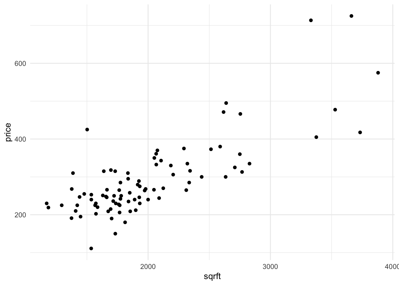
Create a scatterplot of
priceandsqrft. Like every plot you make, ensure that the plot minimally has a title and meaningful axes.Find the correlation between the two variables.
Recall the equation for the slope of the OLS regression line – here you can either use Variance and Covariance, or if you’re bold, the linear algebra. Compute the slope manually (without using
lm())Regress
priceonsqrftusing thelmfunction. This will produce an estimate for the following model:
\[ price = \beta_{0} + \beta_{1} sqrft + e \]

Create a scatterplot that includes the fitted regression.
Interpret what the coefficient means.
- State what features you are allowing to change and what features you’re requiring do not change.
- For each additional square foot, how much more (or less) is the house worth?
- Estimate a new model (and save it into another object) that includes the size of the lot and whether the house is a colonial. This will estimate the model:
\[ price = \beta_{0} + \beta_{1} sqrft + \beta_{2} lotsize + \beta_{3} colonial? + e \]
- BUT BEFORE YOU DO, make a prediction: What do you think is going to happen to the coefficient that relates square footage and price?
- Will the coefficient increase, decrease, or stay the same?
- Compute the sample correlation between \(X\) and \(e_i\). What guarantees do we have from the book about this correlation? Does the data seem to bear this out?