11.6 R Exercise
11.6.1 Omitted Variable Bias in R
The file htv.RData contains data from the 1991 National Longitudinal Survey of Youth, provided by Wooldridge. All people in the sample are males age 26 to 34. The data is interesting here, because it includes education, stored in the variable educ, and also a score on an ability test, stored in the variable abil.
Code
load('./data/htv.RData')

data <- data %>%
  rename(
    ability    = abil,
    education  = educ,
    north_east = ne,
    north_cent = nc,
    potential_experience = exper,
    edu_mother = motheduc,
    edu_father = fatheduc,
    divorce_14 = brkhme14,
    siblings   = sibs,
    tuition_17 = tuit17,
    tuition_18 = tuit18) %>%
  mutate(
    education_f = cut(education, breaks = c(0,12,16,100))) %>%
  select(-c(ctuit, expersq, lwage))

glimpse(data)
## Rows: 1,230
## Columns: 21
## $ wage <dbl> 12.019231, 8.912656, 15.514334, 13.333333, 11.070…
## $ ability <dbl> 5.0277381, 2.0371704, 2.4758952, 3.6092398, 2.636…
## $ education <int> 15, 13, 15, 15, 13, 18, 13, 12, 13, 12, 12, 12, 1…
## $ north_east <int> 0, 1, 1, 1, 1, 1, 1, 0, 1, 1, 1, 1, 0, 1, 1, 1, 1…
## $ north_cent <int> 0, 0, 0, 0, 0, 0, 0, 0, 0, 0, 0, 0, 0, 0, 0, 0, 0…
## $ west <int> 1, 0, 0, 0, 0, 0, 0, 0, 0, 0, 0, 0, 1, 0, 0, 0, 0…
## $ south <int> 0, 0, 0, 0, 0, 0, 0, 1, 0, 0, 0, 0, 0, 0, 0, 0, 0…
## $ potential_experience <int> 9, 8, 11, 6, 15, 8, 13, 14, 9, 9, 13, 14, 4, 8, 7…
## $ edu_mother <int> 12, 12, 12, 12, 12, 12, 13, 12, 10, 14, 9, 12, 17…
## $ edu_father <int> 12, 10, 16, 12, 15, 12, 12, 12, 12, 12, 10, 16, 1…
## $ divorce_14 <int> 0, 1, 0, 0, 1, 0, 0, 1, 1, 0, 1, 0, 0, 0, 0, 0, 0…
## $ siblings <int> 1, 4, 2, 1, 2, 2, 5, 4, 3, 1, 2, 1, 1, 3, 2, 2, 1…
## $ urban <int> 1, 1, 1, 1, 1, 1, 1, 0, 1, 1, 1, 0, 1, 1, 1, 1, 1…
## $ ne18 <int> 1, 1, 1, 1, 1, 1, 1, 1, 1, 1, 1, 1, 1, 1, 1, 1, 1…
## $ nc18 <int> 0, 0, 0, 0, 0, 0, 0, 0, 0, 0, 0, 0, 0, 0, 0, 0, 0…
## $ south18 <int> 0, 0, 0, 0, 0, 0, 0, 0, 0, 0, 0, 0, 0, 0, 0, 0, 0…
## $ west18 <int> 0, 0, 0, 0, 0, 0, 0, 0, 0, 0, 0, 0, 0, 0, 0, 0, 0…
## $ urban18 <int> 1, 1, 1, 1, 1, 1, 1, 1, 1, 1, 1, 1, 1, 1, 1, 1, 1…
## $ tuition_17 <dbl> 7.582914, 8.595144, 7.311346, 9.499537, 7.311346,…
## $ tuition_18 <dbl> 7.260242, 9.499537, 7.311346, 10.162070, 7.311346…
## $ education_f <fct> "(12,16]", "(12,16]", "(12,16]", "(12,16]", "(12,…Code
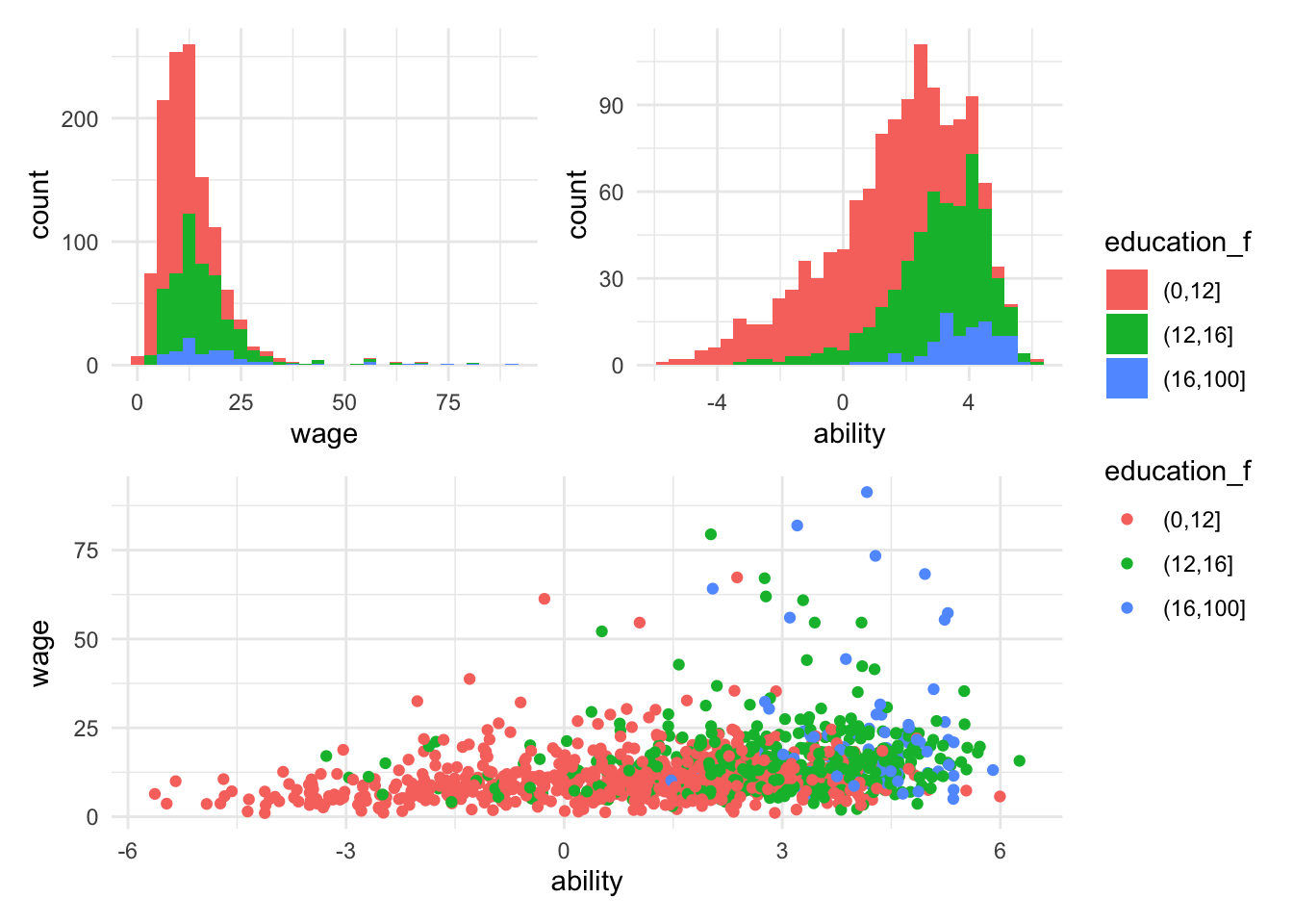
wage_plot <- data %>%
  ggplot() +
  aes(x=wage, fill=education_f) +
  geom_histogram(bins=30)
ability_plot <- data %>%
  ggplot() +
  aes(x=ability, fill=education_f) +
  geom_histogram(bins=30)
wage_by_ability_plot <- data %>%
  ggplot() +
  aes(x=ability, y=wage, color=education_f) +
  geom_point()


(wage_plot | ability_plot) /
  wage_by_ability_plot +
  plot_layout(guides = 'collect')
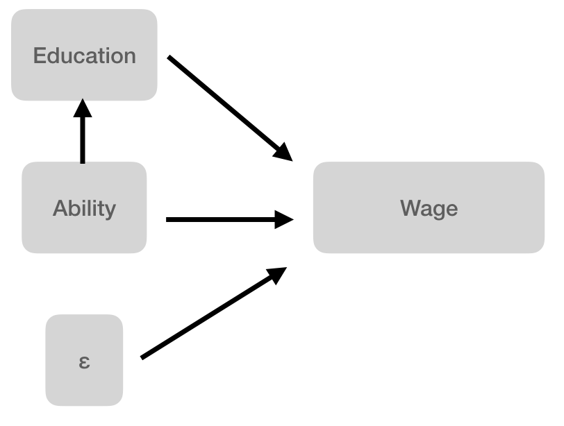
Assume that the true model is,

11.6.2 Questions:
- Are we able to directly measure ability? If so, how would you propose to measure it?
- If not, what do we measure and how is this measurement related to ability? And there is a lot of evidence to suggest that standardized tests are not a very good proxy. But for now, let’s pretend that we really are measuring ability.
- Using R, estimate (a) the true model, and (b) the regression of ability on education.
- Write down the expression for what omitted variable bias would be if you couldn’t measure ability.
- Add this omitted variable bias to the coefficient for education to see what it would be.
- Now evaluate your previous result by fitting the model, \[wage = \alpha_0 + \alpha_1 educ + w\]
- Does the coefficient for the relationship between education and wages match what you estimated earlier?
- Why or why not?
- Reflect on your results:
- What does the direction of omitted variable bias suggest about OLS estimates of returns to education?
- What does this suggest about the reported statistical significance of education?