7.9 The Questions

7.9.1 Set 1

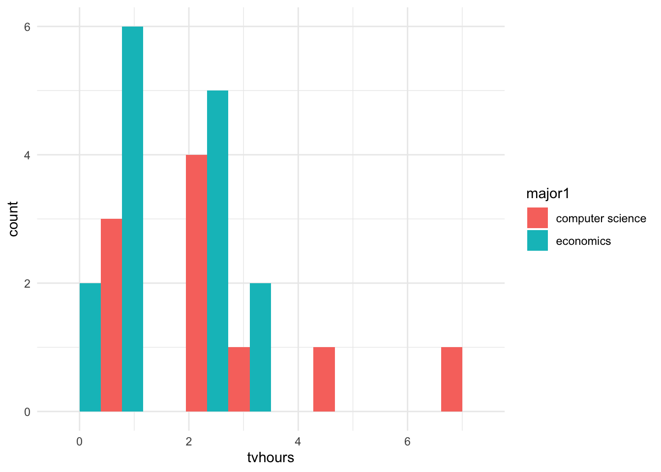
Do economics majors watch more or less TV than computer science majors?

Code

GSS %>% 
  filter(major1 %in% c('computer science', 'economics')) %>% 
  ggplot() + 
  aes(x = tvhours, fill = major1) + 
  geom_histogram(bins = 10, position = 'dodge')

## Warning: Removed 11 rows containing non-finite values (`stat_bin()`).

What kinds of tests could be reasonable to conduct? For what part of the data would we conduct these tests?

Code

## The assumptions about the data drive us to the correct test. 
## But, let's ask all the tests that could *possibly* make sense, and see how 
##     matching or mis-matching assumptions changes what we learn. 

## Answers are in the next chunk... but don't jump to them right away.

Do Americans with pets watch more or less TV than Americans without pets?

7.9.2 Set 2

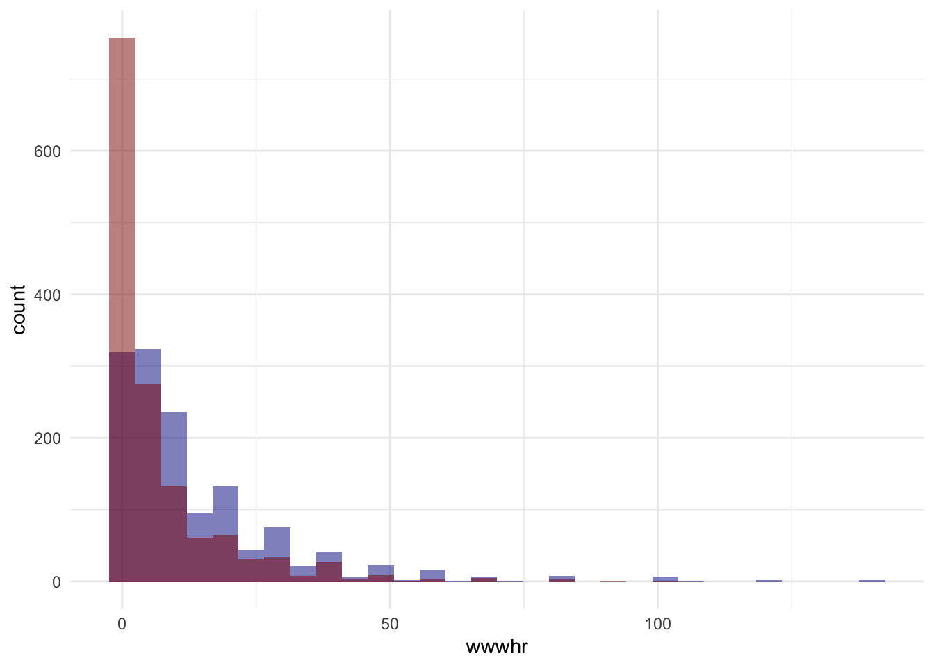
Do Americans spend more time emailing or using the web?

Code

GSS %>% 
  select(wwwhr, emailhr) %>% 
  drop_na() %$% 
  t.test(x = wwwhr, y = emailhr, paired = TRUE)

## 
##  Paired t-test
## 
## data:  wwwhr and emailhr
## t = 13.44, df = 1360, p-value < 2.2e-16
## alternative hypothesis: true mean difference is not equal to 0
## 95 percent confidence interval:
##  5.530219 7.420553
## sample estimates:
## mean difference 
##        6.475386

Code

GSS %>% 
  ggplot() + 
  geom_histogram(aes(x = wwwhr),   fill = 'darkblue', alpha = 0.5) + 
  geom_histogram(aes(x = emailhr), fill = 'darkred',  alpha = 0.5)

## `stat_bin()` using `bins = 30`. Pick better value with `binwidth`.

## Warning: Removed 986 rows containing non-finite values (`stat_bin()`).

## `stat_bin()` using `bins = 30`. Pick better value with `binwidth`.

## Warning: Removed 929 rows containing non-finite values (`stat_bin()`).

Code

t.test(
  x = GSS$wwwhr, 
  y = GSS$emailhr, 
  paired = FALSE
)

## 
##  Welch Two Sample t-test
## 
## data:  GSS$wwwhr and GSS$emailhr
## t = 12.073, df = 2398.5, p-value < 2.2e-16
## alternative hypothesis: true difference in means is not equal to 0
## 95 percent confidence interval:
##  5.657397 7.851614
## sample estimates:
## mean of x mean of y 
## 13.906021  7.151515

Do Americans spend more evenings with neighbors or with relatives?

Code

wilcox_test_data <- GSS %>% 
  select(socrel, socommun) %>%
  mutate(
    family_ordered = factor(
      x      = socrel, 
      levels = c('almost daily', 'sev times a week', 
                 'sev times a mnth', 'once a month',
                 'sev times a year', 'once a year', 'never')),
    friends_ordered = factor(
      x      = socommun, 
      levels = c('almost daily', 'sev times a week', 
                 'sev times a mnth', 'once a month',
                 'sev times a year', 'once a year', 'never')))

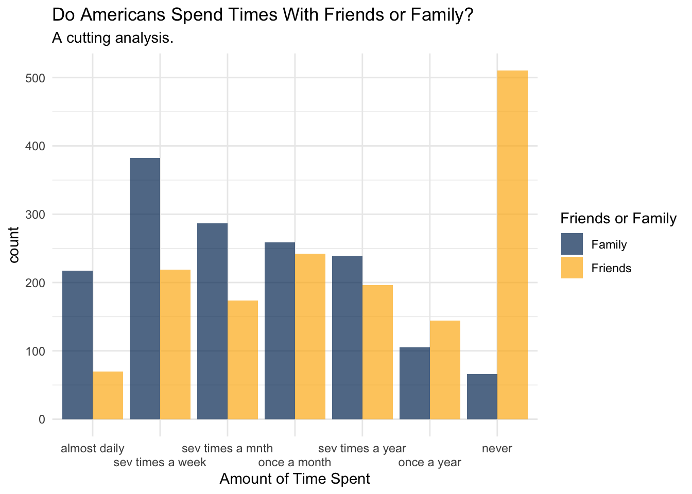
To begin this investigation, we’ve got to look at the data and see what is in it. If you look below, you’ll note that it sure seems that people are spending more time with their family… erp, actually no. They’re “hanging out” with their friends rather than taking their mother out to dinner.

Code

wilcox_test_data %>% 
  select(friends_ordered, family_ordered) %>% 
  rename(
    Friends = friends_ordered, 
    Family  = family_ordered
  ) %>% 
  drop_na() %>% 
  pivot_longer(cols = c(Friends, Family)) %>%   
  ggplot() + 
    aes(x=value, fill=name) + 
    geom_histogram(stat='count', position='dodge', alpha=0.7) + 
  scale_fill_manual(values = c('#003262', '#FDB515')) + 
  labs(
    title    = 'Do Americans Spend Times With Friends or Family?',
    subtitle = 'A cutting analysis.', 
    fill     = 'Friends or Family', 
    x        = 'Amount of Time Spent') + 
  scale_x_discrete(guide = guide_axis(n.dodge = 2)) +
  theme_minimal()

## Warning in geom_histogram(stat = "count", position = "dodge", alpha = 0.7):
## Ignoring unknown parameters: `binwidth`, `bins`, and `pad`

With this plot created, we can ask if what we observe in the plot is the produce of what could just be sampling error, or if this is something that was unlikely to arise due if the null hypothesis were true. What is the null hypothesis? Well, lets suppose that if we didn’t know anything about the data that we would expect there to be no difference between the amount of time spent with friends or families.

Code

## risky choice -- casting the factor to a numeric without checking what happens.
wilcox_test_data %$% 
  wilcox.test(
    x = as.numeric(family_ordered), 
    y = as.numeric(friends_ordered),
    paired = FALSE
  )

## 
##  Wilcoxon rank sum test with continuity correction
## 
## data:  as.numeric(family_ordered) and as.numeric(friends_ordered)
## W = 716676, p-value < 2.2e-16
## alternative hypothesis: true location shift is not equal to 0

7.9.3 Set 3

Are Americans that own guns or Americans that don’t own guns more likely to have pets?
Are Americans with pets happier than Americans without pets?

7.9.4 Apply to a New Type of Data

Is there a relationship between college major and gun ownership?