5.6 Understanding Sampling Distributions

How do sampling distributions change as we add data to them? This is going to both motivate convergence, and also play forward into the Central Limit Theorem. Let’s work through an example that begins with a case that we can think through and draw ourselves. Once we feel pretty good about the very small sample, then we will rely on R to do the work when we expand the example beyond what we can draw ourselves.

Suppose that \(X\) is a Bernoulli random variable representing an unfair coin. Suppose that the coin has a 70% chance of coming up heads: \(P(X=1) = 0.7\).

To begin, suppose that you take that coin, and you toss it two times: you have an iid sample of size 2, \((X_1,X_2)\).
What is the sampling distribution of the sample average, of this sample of size two?
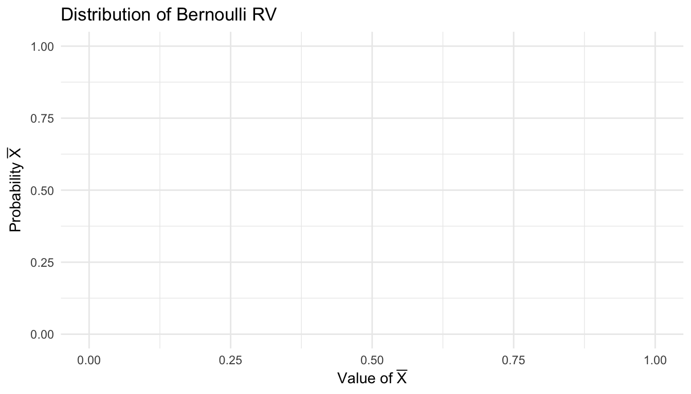
On the axes below, draw the probability distribution of \(\overline X = \frac{X_1+X_2}{2}\).

What if you took four samples? What would the sampling distribution of \(\overline{X}\) look like? Draw this onto the axis above.
Explain the difference between a population distribution and the sampling distribution of a statistic.
Why do we want to know things about the sampling distribution of a statistic?

We are going to write a function that, essentially, just wraps a built-in function with a new name and new function arguments. This is, generally, bad coding practice – because it is changing the default lexicon than a collaborator needs to be aware of – but it is useful for teaching purposes here.

The number_of_simulations argument to the toss_coin function basically just adjusts the precision of our simulation study.
Let’s set, and keep this at \(1000\) simulations. But, if you’re curious, you could set this to be \(5\), or \(10\) and evaluate what happens.

Code

toss_coin <- function(
    number_of_simulations=1000, 
    number_of_tosses=2, 
    prob_heads=0.7) { 
  
  ## number of simulations is just how many times we want to re-run the experiment
  ## number of tosses is the number of coins we're going to toss.
  number_of_heads <- rbinom(n=number_of_simulations, size=number_of_tosses, prob=prob_heads)
  sample_average  <- number_of_heads / number_of_tosses
  return(sample_average)
}

toss_coin(number_of_simulations=10, number_of_tosses=2, prob_heads=0.7)

##  [1] 1.0 0.5 1.0 0.5 0.5 0.5 0.5 0.5 1.0 1.0

Code

ncoins <- 10

coin_result_005 <- toss_coin(
  number_of_simulations = 10000,
  number_of_tosses = ncoins, 
  prob_heads = 0.005
  )

coin_result_05 <- toss_coin(
  number_of_simulations = 10000,
  number_of_tosses = ncoins, 
  prob_heads = 0.5
  )

plot_005 <- ggplot() + 
    aes(x=coin_result_005) + 
    geom_histogram(bins=50) + 
    geom_vline(xintercept=0.005, color='#003262', linewidth=2)

plot_05 <- ggplot() + 
    aes(x=coin_result_05) + 
    geom_histogram(bins=50) + 
    geom_vline(xintercept=0.5, color='#003262', linewidth=2)

plot_005 / 
  plot_05

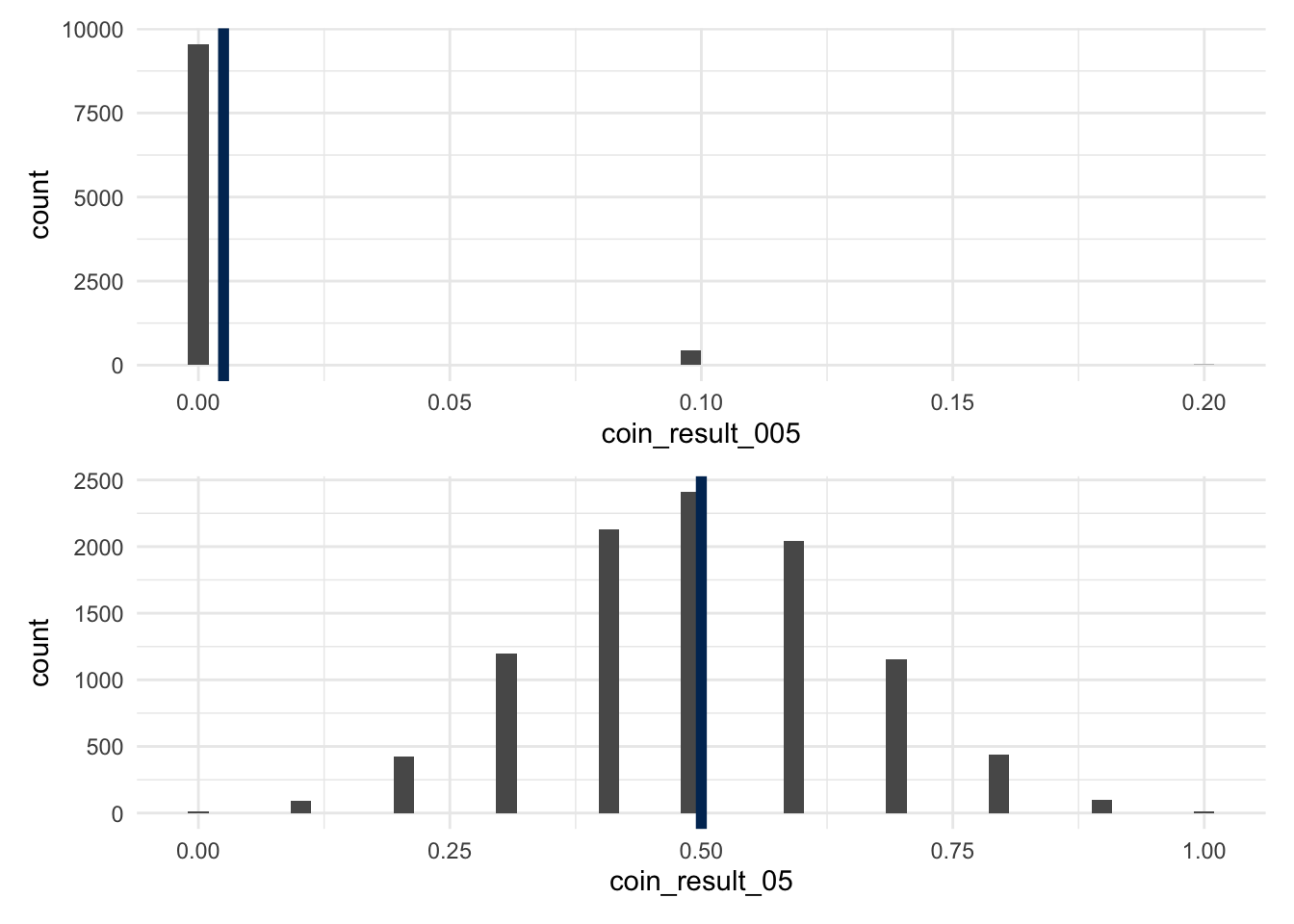
In the plot that you have drawn above, pick some value, \(\epsilon\) that is the distance away from the true expected value of this distribution.

What proportion of the sampling distribution is further away than \(E[X] \pm \epsilon\)?
When we toss the coin only two times, we can quickly draw out the distribution of \(\overline{X}\), and can form a statement about the \(P(E[X] - \epsilon \leq \overline{X} \leq E[X] + \epsilon)\).
What if we toss the coin ten times? We can still use the IID nature of the coin to figure out the true \(P(\overline{X} = 0), P(\overline{X} = 1), \dots, P(\overline{X} = 10)\), but it is going to start to take some time. This is where we rely on the simulation to start speeding up our learning.
As we toss more and more coins, \(\overline X_{(100)} \rightarrow \overline X_{(10000)}\) what will the value of \(\overline X\) get closer to? What law generates this, and why does this law generate this result?