3.9 Write Code

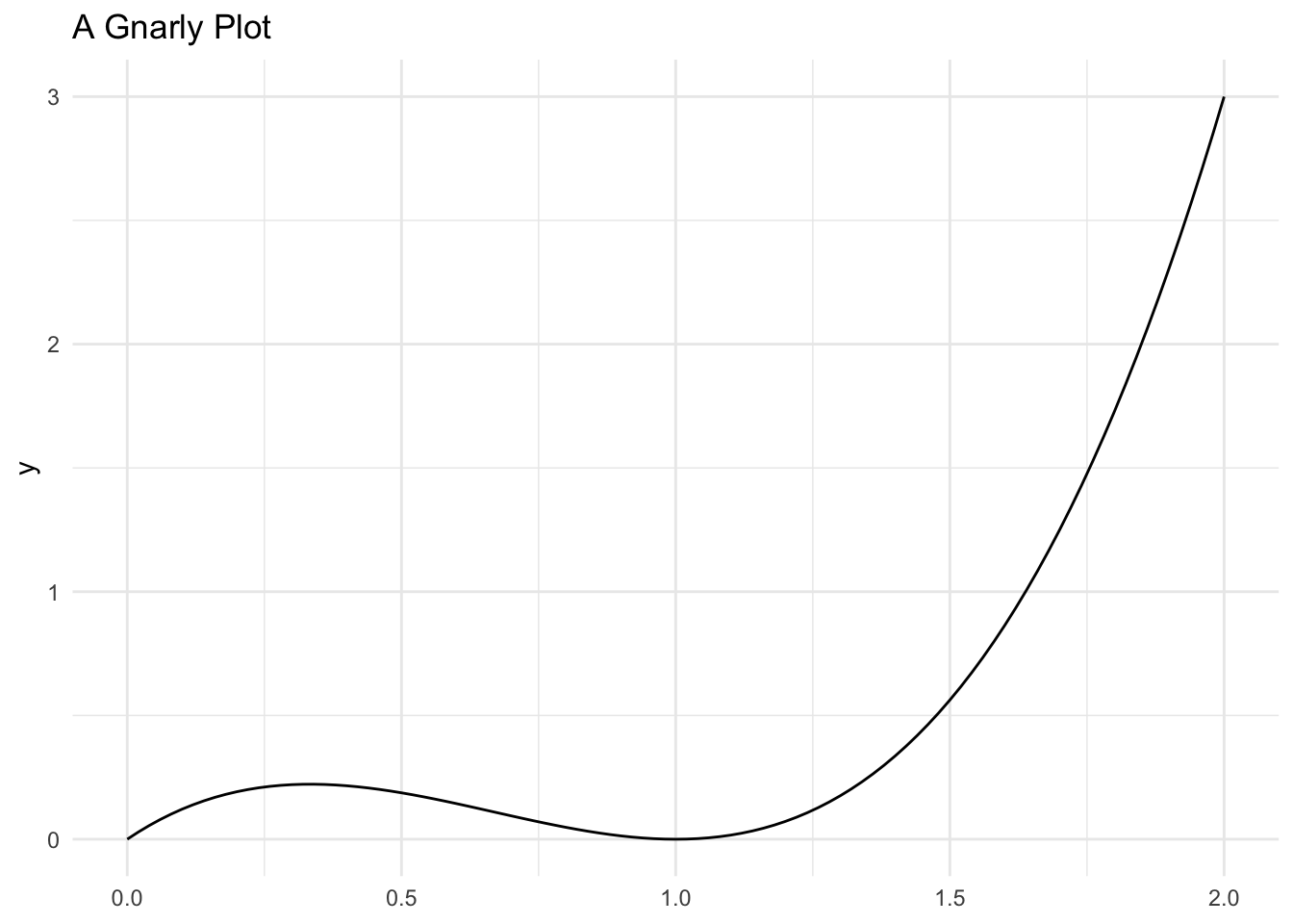
Suppose that you have a random variable with a gnarly probability distribution function:

\[ f_{X}(x) = \frac{3*\left(x - 2x^2 + x^3\right)}{2}, 0\leq x\leq 2 \]

If you had to pick a single value that minimizes the \(MSE\) of this function, what would it be?

• First, how would you approach this problem analytically. By this, we mean, “how would you solve this with the closed form answer?
• Second, how might you approach this problem computationally. By this, we mean, “how might you write code that would produce a numeric approximation of the closed form solution?” Don’t worry about actually writing the code – we’ll have done that for you, but what is the process (called in our world, algorithm) that you would use to determine the value that produces the smallest \(MSE\)?

Code

pdf_fun <- function(x) { 
  (3/2)*(x - (2*x^2) + x^3)
}

Code

support <- seq(from=0, to=2, by=0.01)

Code

ggplot() + 
  geom_function(fun = pdf_fun) + 
  xlim(min(support), max(support)) + 
  labs(
    title = "A Gnarly Plot"
  )

Code

expected_value <- function(value, prob){
  sum(value * prob)
}

mse <- function(c) { 
  expected_value(
    value = (support - c)^2, 
    prob  = pdf_fun(support)
  )  
}

mpe <- function(c, power) { 
  expected_value(
    value = (support - c)^power, 
    prob  = pdf_fun(support)
  )
}

Code

mean_absolute_error <- function(c) { 
  x_values <- pdf_fun(support)
  mae_     <- mean(abs(x_values - c))
}

mean_square_error <- function(c) { 
  x_values <- pdf_fun(support)
  mse_     <- sum(((x_values - c)^2) * x_values)
  return(mse_)
}

mean_cubic_error <- function(c) { 
  x_values <- pdf_fun(support) 
  mce_     <- mean((x_values - c)^3)
}

mean_quadratic_error <- function(c) { 
  x_values <- pdf_fun(support)
  mqe_     <- mean((x_values - c)^4)
  return(mqe_)
}

mean_power_error <- function(c, power) { 
  x_values <- pdf_fun(support)
  m_power_e_     <- mean((x_values - c)^power)
  return(m_power_e_)
}

Code

mean_absolute_error  <- Vectorize(mean_absolute_error)
mean_square_error    <- Vectorize(mean_square_error)
mean_cubic_error     <- Vectorize(mean_cubic_error)
mean_quadratic_error <- Vectorize(mean_quadratic_error)
mean_power_error     <- Vectorize(mean_power_error)

Code

mae_ <- mean_absolute_error(
  c = support
)
mse_ <- mean_square_error(
  c = support
  )
mce_ <- mean_cubic_error(
  c = support
)
mqe_ <- mean_quadratic_error(
  c = support
)

Code

absolute_error_ <- optim(
  par = 0, 
  fn = mean_absolute_error, 
  method = 'Brent', 
  lower = 0, upper = 2
  )$par

squared_error_ <- optim(
  par = 0, 
  fn = mean_square_error, 
  method = "Brent", 
  lower = 0, upper = 2
  )$par
cubic_error_ <- optim(
  par = 0, 
  fn = mean_cubic_error, 
  method = "Brent", 
  lower = 0, upper = 2
  )$par
quadratic_error_ <- optim(
  par = 0, 
  fn = mean_quadratic_error, 
  method = "Brent", 
  lower = 0, upper = 2
  )$par

Code

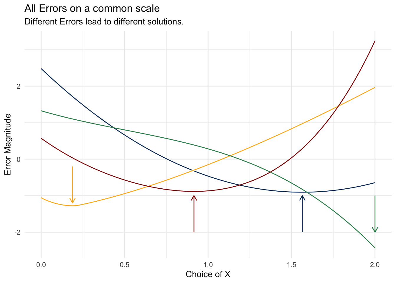
all_plots <- ggplot() + 
  ## add lines 
  geom_line(aes(x=support, y=scale(mse_)), color = "#003262")  + 
  geom_line(aes(x=support, y=scale(mae_)), color = "#FDB515")  + 
  geom_line(aes(x=support, y=scale(mce_)), color = "seagreen") + 
  geom_line(aes(x=support, y=scale(mqe_)), color = "darkred")  +
  ## add optimal solution indicators
  geom_segment(
    aes(x = squared_error_, 
    xend = squared_error_, 
    y = -2, 
    yend = -1), 
    arrow = arrow(length = unit(0.25, "cm")),
    color = "#003262")  + 
  geom_segment(
    aes(x = absolute_error_, 
    xend = absolute_error_, 
    y = -.2, 
    yend = -1.2), 
    arrow = arrow(length = unit(0.25, "cm")),
    color = "#FDB515")  + 
  geom_segment(
    aes(x = cubic_error_, 
    xend = cubic_error_, 
    y = -1, 
    yend = -2), 
    arrow = arrow(length = unit(0.25, "cm")),
    color = "seagreen")  + 
  geom_segment(
    aes(x = quadratic_error_, 
    xend = quadratic_error_, 
    y = -2, 
    yend = -1), 
    arrow = arrow(length = unit(0.25, "cm")),
    color = "darkred")  + 
  labs(
    title    = "All Errors on a common scale", 
    subtitle = "Different Errors lead to different solutions.", 
    y        = "Error Magnitude", 
    x        = "Choice of X"
  )

all_plots