9.7 R Exercise
Real Estate in Boston
The file hprice1.RData contains 88 observations of homes in the Boston area, taken from the real estate pages of the Boston Globe during 1990. This data was provided by Wooldridge.
Last week, we fit a regression of price on square feet.
## [1] 86Can you use the pieces that you’re familiar with to produce a p-value using robust standard errors?
Code
regression_p_value <- function(model, variable) {
  ## this function takes a model
  ## and computes a test-statistic,
  ## then compares that test-statistic against the
  ## appropriate t-distribution

  ## you can use the following helper functions:
  ##  - coef()
  ##  - vcovHC()
  df <- model$df.residual

  # numerator   <- 'fill this in'
  # denominator <- 'fill this in'

  numerator   <- coef(model)[variable]
  denominator <- sqrt(diag(vcovHC(model)))[variable]

  test_stat_  <- numerator / denominator
  p_val_      <- 'fill this in'
  p_val_      <- pt(test_stat_, df = df, lower.tail = FALSE) * 2

  return(p_val_)
  }
If you want to confirm that what you have written is correct, you can compare against the value that you receive from the line below.
##
## t test of coefficients:
##
##              Estimate Std. Error t value  Pr(>|t|)
## (Intercept) 11.204145  39.450563  0.2840    0.7771
## sqrft        0.140211   0.021111  6.6417 2.673e-09 ***
## ---
## Signif. codes:  0 '***' 0.001 '**' 0.01 '*' 0.05 '.' 0.1 ' ' 1
Code
p_value_ <- broom::tidy(coeftest(model_one, vcov. = vcovHC(model_one))) %>%
  filter(term == 'sqrft') %>%
  select('p.value') %>%
  as.numeric()

test_that(
  'test that hand coded p-value is the same as the pre-rolled',
  expect_equal(
    object   = as.numeric(regression_p_value(model_one, 'sqrft')),
    expected = p_value_
  )
)
## Test passed 🎊Questions
- Estimate a new model (and save it into another object) that includes the size of the lot and whether the house is a colonial. This will estimate the model:
\[ price = \beta_{0} + \beta_{1} sqrft + \beta_{2} lotsize + \beta_{3} colonial? + e \]
- BUT BEFORE YOU DO, make a prediction: What do you think is going to happen to the coefficient that relates square footage and price?
- Will the coefficient increase, decrease, or stay the same?
- Will the uncertainty about the coefficient increase, decrease, or stay the same?
- Conduct an F-test that evaluates whether the model as a whole does better when the coefficients on
colonialandlotsizeare allowed to estimate freely, or instead are restricted to be zero (i.e. \(\beta_{2} = \beta_{3} = 0\).
Use the function
vcovHCfrom thesandwichpackage to estimate (a) the the heteroskedastic consistent (i.e. “robust”) variance covariance matrix; and (b) the robust standard errors for the intercept and slope of this regression. Recall, what is the relationship between the VCOV and SE in a regression?Perform a hypothesis test to check whether the population relationship between
sqrftandpriceis zero. Usecoeftest()with the robust standard errors computed above.Use the robust standard error and
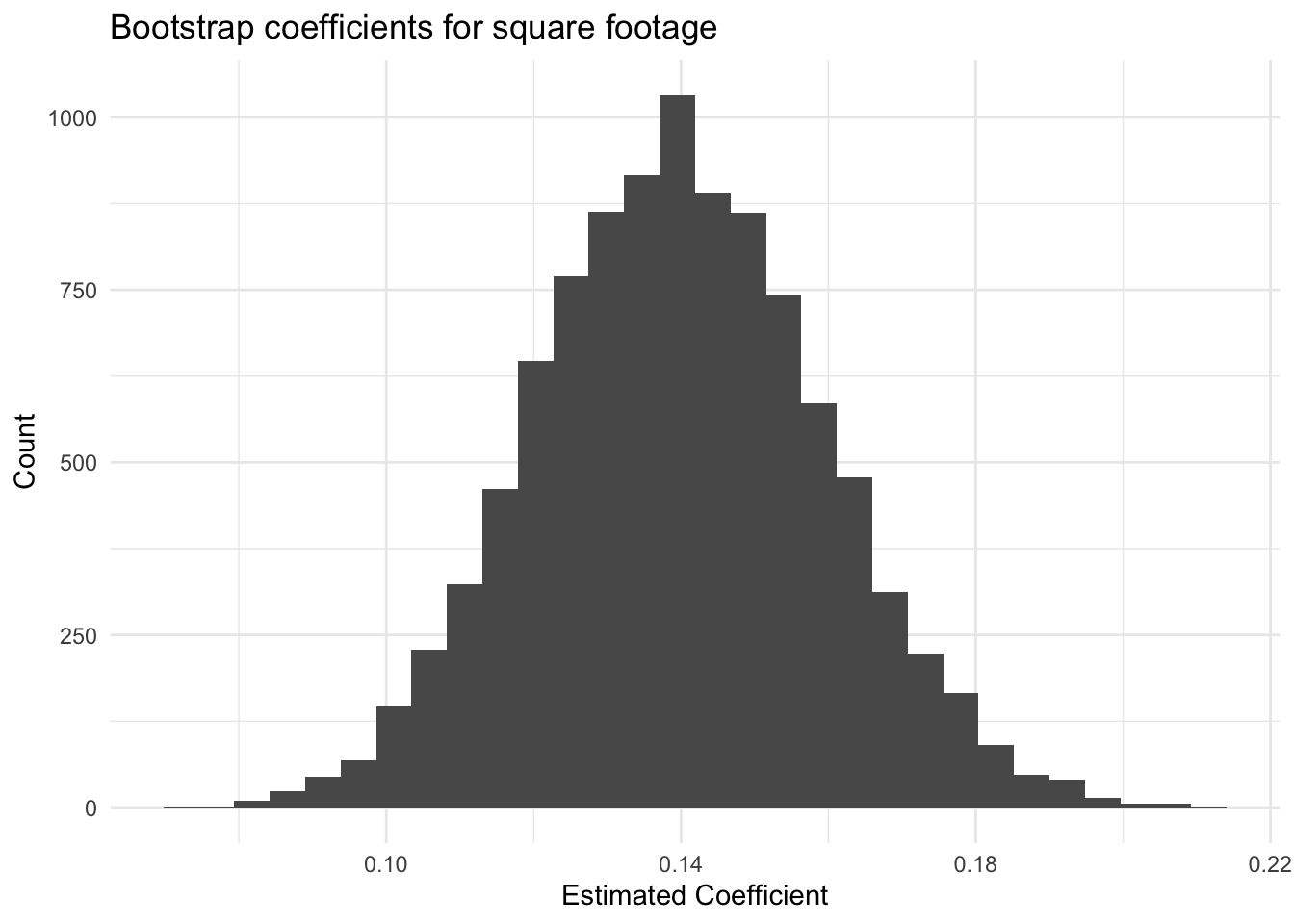
qtto compute a 95% confidence interval for the coefficientsqrftin the second model that you estimated. \(price = \beta_{0} + \beta_{1} sqrft + \beta_{2} lotsize + \beta_{3} colonial\).Bootstrap. The book very quickly talks about bootstrapping which is the process of sampling with replacement and fitting a model. The idea behind the bootstrap is that since the data is generated via an iid sample from the population, that you can simulate re-running your analysis by drawing repeated samples from the data that you have.
Below is code that will conduct a boostrapping estimator of the uncertainty of the sqrft variable when lotsize and colonial are included in the model.
Code
bootstrap_sqft <- function(d = data, number_of_bootstraps = 1000) {
  number_of_rows <- nrow(d)

    coef_sqft <- rep(NA, number_of_bootstraps)

    for(i in 1:number_of_bootstraps) {
      bootstrap_data <- d[sample(x=1:number_of_rows, size=number_of_rows, replace=TRUE), ]
      estimated_model <- lm(price ~ sqrft, data = bootstrap_data)
      coef_sqft[i]    <- coef(estimated_model)['sqrft']
    }
  return(coef_sqft)
}With this, it is possible to plot the distribution of these regression coefficients:
Code
## `stat_bin()` using `bins = 30`. Pick better value with `binwidth`.
Compute the standard deviation of the bootstrapped regression coefficients. How does this compare to the robust standard errors you computed above?
##
## t test of coefficients:
##
##              Estimate Std. Error t value  Pr(>|t|)
## (Intercept) 11.204145  39.450563  0.2840    0.7771
## sqrft        0.140211   0.021111  6.6417 2.673e-09 ***
## ---
## Signif. codes: 0 '***' 0.001 '**' 0.01 '*' 0.05 '.' 0.1 ' ' 1## [1] 0.01959866